Foursquare S3 Data
Landscaping Businesses in the US
By Steve Ewing
November 20, 2024
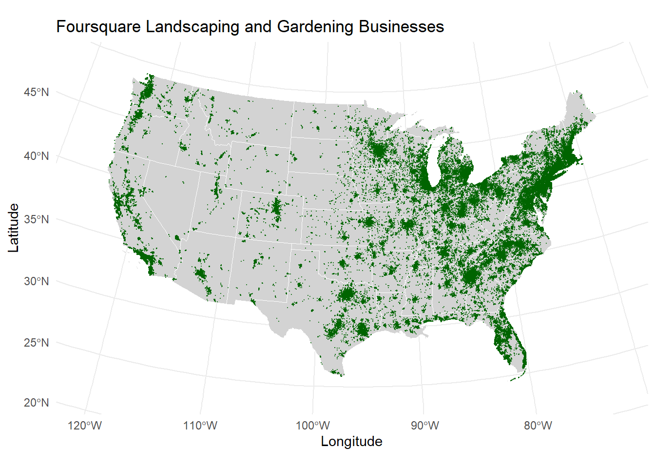
Foursquare open sourced their database in the form of Parquet files stored in an S3 bucket. This data can be queried using DuckDB. In this post, I will show how to query the Foursquare data to get all the landscaping businesses in the US.
First find how they label landscaping businesses in the data.
# Load the duckdb package
library(duckdb)

# Create a DuckDB connection
con <- dbConnect(duckdb::duckdb())

# Install and load the httpfs extension
dbExecute(con, "INSTALL httpfs;")
## [1] 0
dbExecute(con, "LOAD httpfs;")
## [1] 0
# Set S3 Configuration Options
dbExecute(con, "SET s3_region='us-east-1';")
## [1] 0
dbExecute(con, "SET s3_endpoint='s3.amazonaws.com';")
## [1] 0
dbExecute(con, "SET s3_url_style='path';")
## [1] 0
dbExecute(con, "SET s3_access_key_id='';")
## [1] 0
dbExecute(con, "SET s3_secret_access_key='';")
## [1] 0
# Define the S3 path to a single Parquet file for sampling
s3_path_sample <- "s3://fsq-os-places-us-east-1/release/dt=2024-11-19/places/parquet/places-00000.snappy.parquet"

# Define the query to extract distinct category labels containing 'Landscape'
category_query <- paste0("
SELECT DISTINCT label_value
FROM (
    SELECT UNNEST(t.fsq_category_labels) AS label_value
    FROM '", s3_path_sample, "' AS t
    WHERE t.fsq_category_labels IS NOT NULL
) AS labels
WHERE label_value LIKE '%Landscape%'
")

# Execute the query
category_labels <- dbGetQuery(con, category_query)

# Print the resulting category labels
print(category_labels)
##                                                                               label_value
## 1 Business and Professional Services > Home Improvement Service > Landscaper and Gardener
Get all the Landscaper and Gardener business data from Foursquare using duck db.
# Create a DuckDB connection
con <- dbConnect(duckdb::duckdb())

# Install and load the httpfs extension
dbExecute(con, "INSTALL httpfs;")
dbExecute(con, "LOAD httpfs;")

# Set S3 Configuration Options
dbExecute(con, "SET s3_region='us-east-1';")
dbExecute(con, "SET s3_endpoint='s3.amazonaws.com';")
dbExecute(con, "SET s3_url_style='path';")
dbExecute(con, "SET s3_access_key_id='';")
dbExecute(con, "SET s3_secret_access_key='';")

# Define the exact category label
label <- 'Business and Professional Services > Home Improvement Service > Landscaper and Gardener'

# Define the S3 path to include all Parquet files
s3_path_all <- "s3://fsq-os-places-us-east-1/release/dt=2024-11-19/places/parquet/*.parquet"

# Define the main query using array_contains
query <- paste0("
SELECT *
FROM '", s3_path_all, "' AS t
WHERE t.country = 'US'
  AND t.fsq_category_labels IS NOT NULL
  AND array_contains(t.fsq_category_labels, '", label, "')
")

# Specify the output file name
output_file <- "landscaping_and_gardening_businesses.csv"

# Execute the query and write results to a CSV file
copy_query <- paste0("
COPY (", query, ")
TO '", output_file, "'
WITH (FORMAT CSV, HEADER TRUE)
")

dbExecute(con, copy_query)

# Disconnect from the database
dbDisconnect(con)
Load the data into R and display the first few rows.
Get the map using Tigris
# Install and load packages
library(dplyr)
library(ggplot2)
library(tigris)
library(sf)

# Connect to DuckDB
con <- dbConnect(duckdb::duckdb(), dbdir = ":memory:")

# Read the CSV file into DuckDB
dbExecute(con, "
    CREATE TABLE landscaping_data AS
    SELECT * FROM read_csv_auto('landscaping_and_gardening_businesses.csv')
")
## [1] 100927
# Reference the DuckDB table using dplyr
landscaping_tbl <- tbl(con, "landscaping_data")

# Prepare the data
landscaping_data <- landscaping_tbl %>%
  filter(!is.na(latitude), !is.na(longitude), is.na(date_closed)) %>%
  select(name, latitude, longitude, address, locality, region) %>%
  collect() %>%
  mutate(
    latitude = as.numeric(latitude),
    longitude = as.numeric(longitude)
  )

# Convert the data frame to an sf object
landscaping_sf <- st_as_sf(
  landscaping_data,
  coords = c("longitude", "latitude"),
  crs = 4326,  # Original CRS (WGS84)
  remove = FALSE
)

# Transform to Albers Equal Area Conic projection (EPSG:5070)
landscaping_sf <- st_transform(landscaping_sf, crs = 5070)

# Get US states shapefile, exclude non-continental states, and transform to the same CRS
options(tigris_use_cache = TRUE)
us_states <- states(cb = TRUE, resolution = "20m", class = "sf") %>%
  # Exclude Alaska, Hawaii, and territories
  filter(!NAME %in% c(
    "Alaska", "Hawaii", "Puerto Rico", "Guam",
    "American Samoa", "Commonwealth of the Northern Mariana Islands",
    "United States Virgin Islands"
  )) %>%
  st_transform(crs = 5070)

# Calculate the bounding box from us_states
bbox <- st_bbox(us_states)

# Optionally, expand the bounding box by 5%
xrange <- bbox["xmax"] - bbox["xmin"]
yrange <- bbox["ymax"] - bbox["ymin"]

bbox_expanded <- bbox
bbox_expanded["xmin"] <- bbox["xmin"] - 0.05 * xrange
bbox_expanded["xmax"] <- bbox["xmax"] + 0.05 * xrange
bbox_expanded["ymin"] <- bbox["ymin"] - 0.05 * yrange
bbox_expanded["ymax"] <- bbox["ymax"] + 0.05 * yrange

# Create the map with the improved CRS and bounding box
ggplot() +
  geom_sf(data = us_states, fill = "lightgray", color = "white") +
  geom_sf(
    data = landscaping_sf,
    color = "darkgreen",
    alpha = 0.7,
    size = 0.1
  ) +
  coord_sf(
    crs = st_crs(5070),
    xlim = c(bbox_expanded["xmin"], bbox_expanded["xmax"]),
    ylim = c(bbox_expanded["ymin"], bbox_expanded["ymax"])
  ) +
  theme_minimal() +
  labs(
    title = "Foursquare Landscaping and Gardening Businesses",
    x = "Longitude",
    y = "Latitude"
  )

# Save the plot (uncomment if you wish to save the plot)
# ggsave("landscaping_businesses_map_albers.png", width = 10, height = 6)

# Disconnect from DuckDB
dbDisconnect(con)

# Delete the .tmp folder if it exists
if (dir.exists(".tmp")) {
  unlink(".tmp", recursive = TRUE, force = TRUE)
}